Calculating analytically solutions to differential equations can be hard and sometimes even impossible. Methods exist for special types of ODEs. One method is to solve the ODE by separation of variables. The idea of substitution is to replace some variable so that the resulting equation has the form of such a special type where a solution exists. In this scenario, I want to look at homogeneous ODEs which have the form
\begin{equation} y'(x) = F\left( \frac{y(x)}{x} \right). \label{eq:homogeneousODE} \end{equation}They can be solved by replacing \(z=\frac{y}{x}\) followed by separation of variables. Equations of this kind have the special property of being invariant against uniform scaling (\(y \rightarrow \alpha \cdot y_1, x \rightarrow \alpha \cdot x_1\)):
\begin{align*} \frac{\alpha \cdot \partial y_1}{\alpha \cdot \partial x_1} &= F\left( \frac{\alpha \cdot y_1}{\alpha \cdot x_1} \right) \\ \frac{\partial y_1}{\partial x_1} &= F\left( \frac{y_1}{x_1} \right) \end{align*}Before analysing what this means, I want to introduce the example from the corresponding Lecture 4: First-order Substitution Methods (MIT OpenCourseWare), which is the source of this article. I derive the substitution process for this example later.
Imagine a small island with a lighthouse built on it. In the surrounding sea is a drug boat which tries to sail silently around the sea raising no attention. But the lighthouse spots the drug boat and targets the boat with its light ray. Panic-stricken the boat tries to escape the light ray. To introduce some mathematics to the situation, we assume that the boat always tries to escape the light ray in a 45° angle. Of course, the lighthouse reacts accordingly and traces the boat back. The following image depicts the situation.
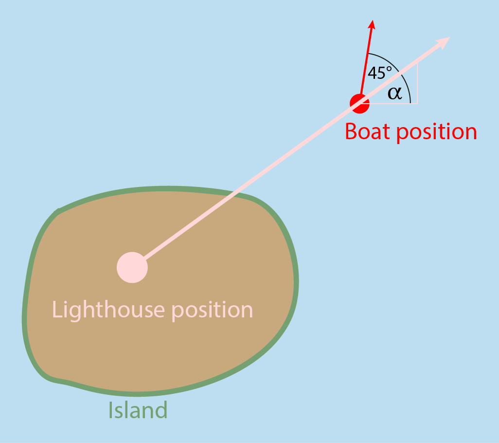
We now want to know the boat's curve, when the light ray always follows the boat directly and the boat, in turn, evades in a 45° angle. We don't model the situation as a parametric curve where the position would depend on time (so no \((x(t), y(t))\) here). This also means that we don't set the velocity of the curve explicitly. Instead, the boat position just depends on the angle of the current light ray. Mathematically, this means that in the boat's curve along the x-y-plane the tangent of the curve is always enclosed in a 45° angle with the light ray crossing the boat's position. \(\alpha\) is the angle of the light ray and when we assume that the lighthouse is placed at the origin so that the slope is just given by the fraction \(\frac{y}{x}\), \(\alpha\) is simply calculated as
\begin{equation*} \tan(\alpha) = \frac{y}{x}. \end{equation*}Now we can define the tangent of the boat's curve, which is given by its slope value
\begin{equation} y'(x) = f(x,y(x)) = \tan(\alpha + 45°) = \frac{\tan(\alpha) + \tan(45°)}{1 - \tan(\alpha) \cdot \tan(45°)} = \frac{\frac{y(x)}{x} + 1}{1 - \frac{y(x)}{x}} = \frac{x + y(x)}{x - y(x)}. \label{eq:slopeBoat} \end{equation}In the first simplification step, a trigonometric addition formula is used. This again can be simplified so that the result fulfils the definition of \eqref{eq:homogeneousODE}. This means that the ODE can be solved by separation of variables if the substitution \(z(x) = \frac{y(x)}{x}\) is made. We want to replace \(y'(x)\), so we first need to calculate the derivative of the substitution equation
\begin{align*} y(x) &= z(x) \cdot x \\ y'(x) &= \frac{\partial y(x)}{\partial x} = z'(x) \cdot x + z(x). \end{align*}Note that we calculate the derivative with respect to \(x\) and not \(y(x)\) (which is a function depending on \(x\) itself). Therefore the product rule was used. Next we substitute and try to separate variables.
\begin{align*} y'(x) &= \frac{x + y(x)}{x - y(x)} \\ z'(x) \cdot x + z(x) &= \frac{x + z(x) \cdot x}{x - z(x) \cdot x} \\ \frac{\partial z(x)}{\partial x} \cdot x &= \frac{1 + z(x)}{1 - z(x)} - z(x) = \frac{1 + z(x)}{1 - z(x)} - \frac{\left( 1-z(x) \right) \cdot z(x)}{1-z(x)} = \frac{1 + z(x) - z(x) + z^2(x)}{1 - z(x)} \\ \frac{\partial z(x)}{\partial x} &= \frac{1 + z^2(x)}{1 - z(x)} \cdot \frac{1}{x} \\ \frac{1 - z(x)}{1 + z^2(x)} \partial z(x) &= \frac{1}{x} \cdot \partial x \\ \int \frac{1 - z(x)}{1 + z^2(x)} \, \mathrm{d} z(x) &= \int \frac{1}{x} \, \mathrm{d} x \\ \tan^{-1}(z(x)) - \frac{1}{2} \cdot \ln \left( z^2(x)+1 \right) &= \ln(x) + C \\ 0 &= -\tan^{-1}\left(z(x)\right) + \frac{1}{2} \cdot \ln \left( z^2(x)+1 \right) + \ln(x) + C \\ 0 &= -\tan^{-1}\left(z(x)\right) + \ln \left( \sqrt{z^2(x) + 1} \cdot x \right) + C \\ 0 &= -\tan^{-1}\left(z(x)\right) + \ln \left( \sqrt{z^2(x) \cdot x^2 + x^2} \right) + C \\ \end{align*}(I used the computer for the integration step) We now have a solution, but we first need to substitute back to get rid of the \(z(x) = \frac{y(x)}{x}\)
\begin{align*} 0 &= -\tan^{-1}\left(\frac{y(x)}{x}\right) + \ln \left( \sqrt{\frac{y^2(x)}{x^2} \cdot x^2 + x^2} \right) + C \\ 0 &= -\tan^{-1}\left(\frac{y(x)}{x}\right) + \ln \left( \sqrt{y^2(x) + x^2} \right) + C \end{align*}Next, I want to set \(C\) to the starting position of the boat by replacing \(x = x_0\) and \(y(x) = y_0\)
\begin{align*} C &= \tan^{-1}\left(\frac{y_0}{x_0}\right) - \ln \left( \sqrt{y_0^2 + x_0^2} \right) \end{align*}The final result is then an implicit function
\begin{equation} 0 = -\tan^{-1}\left( \frac{y}{x} \right) + \ln\left( \sqrt{x^2 + y^2} \right) + \tan^{-1}\left( \frac{y_0}{x_0} \right) - \ln \left( \sqrt{x_0^2 + y_0^2} \right). \label{eq:curveBoat} \end{equation}So, we now have a function where we plug in the starting point \((x_0,y_0)^T\) of the boat and then check every relevant value for \(y\) and \(x\) where the equation is fulfilled. In total, this results in the boat's curve. Since the boat's position always depends on the current light ray from the lighthouse, you can think of the curve being defined by the ray. To clarify this aspect, you can play around with the slope of the ray in the following animation.
As you can see, the boat's curve originates by rotating the light ray. Also, note that there are actually two curves. This is because we can enclose a 45° angle on both sides of the light ray. The right curve encloses the angle with the top right side of the line and the left curve encloses with the bottom right side of the line. Actually, one starting point defines already both curves, but you may want to depict the situation like two drug boats starting at symmetric positions.
I marked the position \((x_c,y_c) = (1,2)\) as “angle checkpoint” to see if the enclosed angle is indeed 45°. To check, we first need the angle of the light ray which is just the angle \(\alpha\) defined above for the given coordinates
\begin{equation*} \phi_{ray} = \tan^{-1}\left( \frac{y_c}{x_c} \right) = \tan^{-1}\left( \frac{2}{1} \right) = 63.43°. \end{equation*}For the angle of the boat, we need its tangent at that position which is given by its slope value. So we only need to plug in the coordinates in the ODE previously defined
\begin{equation*} f(x_c,y_c) = \frac{1 + 2}{1 - 2} = -3. \end{equation*}Forwarding this to \(\tan^{-1}\) results in the angle of the tangent
\begin{equation*} \phi_{tangent} = \tan^{-1}\left(-3\right) + 180° = -71.57° + 180° = 108.43°. \end{equation*}I added 180° so that the resulting angle is positive (enclosed angles can only be in the range \(\left[0°;180°\right[\)). Calculating the difference \( \phi_{tangent} - \phi_{ray} = 108.43° - 63.43° = 45°\) shows indeed the desired result. Of course, this is not only true at the marked point, but rather at any point instead, because that is the way we defined it in \eqref{eq:slopeBoat}.
Another way of visualising \eqref{eq:curveBoat} is to switch to the the polar coordinate system by using \(\theta = \tan^{-1}\left( \frac{y}{x} \right)\) respectively \( r = \sqrt{x^2 + y^2} \)
\begin{align*} 0 &= -\theta + \ln\left( r \right) + \theta_0 - \ln \left( r_0 \right) \\ \ln \left( \frac{r_0}{r} \right) &= -\theta + \theta_0 \\ \frac{r_0}{r} &= e^{-\theta + \theta_0}, \end{align*}and solve by \(r\)
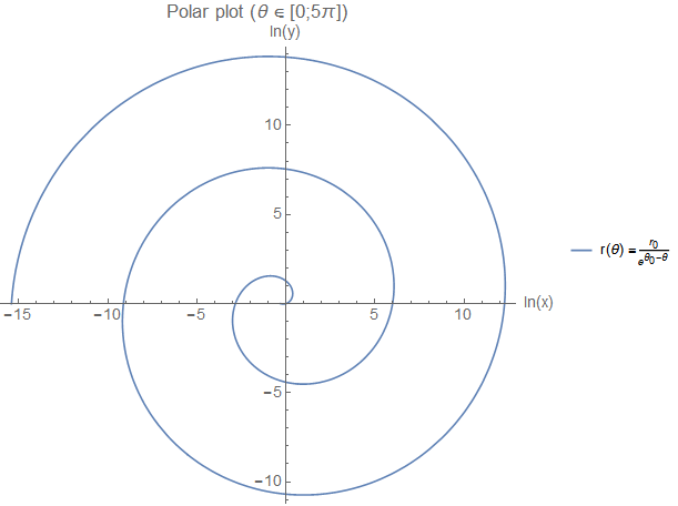
\begin{equation} r\left( \theta \right) = \frac{r_0}{e^{\theta_0 -\theta}}. \label{eq:curveBoatPolar} \end{equation}We can now visualize this function using a polar plot where we move around a (unit) circle and adjust the radius accordingly to \eqref{eq:curveBoatPolar}. The result is a graph which looks like a spiral. Beginning from the starting point the light ray forces the boat to move counter-clockwise in a circle with increasing distance from the island. So, without considering physics (infinity light ray, ...) and realistic human behaviour (escaping strategy of the boat, ...), this cat-and-mouse game lasts forever.
Next, I want to analyse how the curve varies when the starting position of the boat changes. Again, each position of the curve is just given by the corresponding light ray crossing the same position. The curve in total is, therefore, the result of a complete rotation (or multiple like in the polar plot) of the light ray (like above, just with all possible slope values). In the next animation, you can change the starting position manually.
Do you remember the property of scale invariance for a homogeneous ODE introduced in the beginning? Let's have a lock what this means for the current problem. For this, it helps to analyse the different slope values which the equation \(f(x,y)\) produces. This is usually done via a vector field. At sampled positions (\(x_s,y_s\)) in the grid, a vector \((1, f(x_s,y_s))\) is drawn which points in the direction of the slope value at that position (here, the vectors are normalized). So the vector is just a visualization technique to show the value of \(f(x,y)\). Additionally, I added some isoclines where on all points on one line the slope value is identical. This means that all vectors along a line have the same direction (easily checked on the horizontal line).
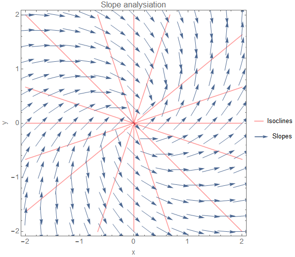
You can check this if you move the boat along the line \(y=x\). This will result in different curves, but the tangent of the boat's starting point is always the same (vertical). Actually, this is already the property of scale invariance: starting from one point, you can scale your point (= moving along an isocline) and always get the same slope value.
List of attached files:
- HomogeneousODESubstitution.nb [PDF] (Mathematica notebook including the visualizations and calculations of this article)